Dataset, MSK COVID-19 12 July 2021
Contents
#
This is a daily report on COVID-19 Moscow dataset. Code source for this report is here.
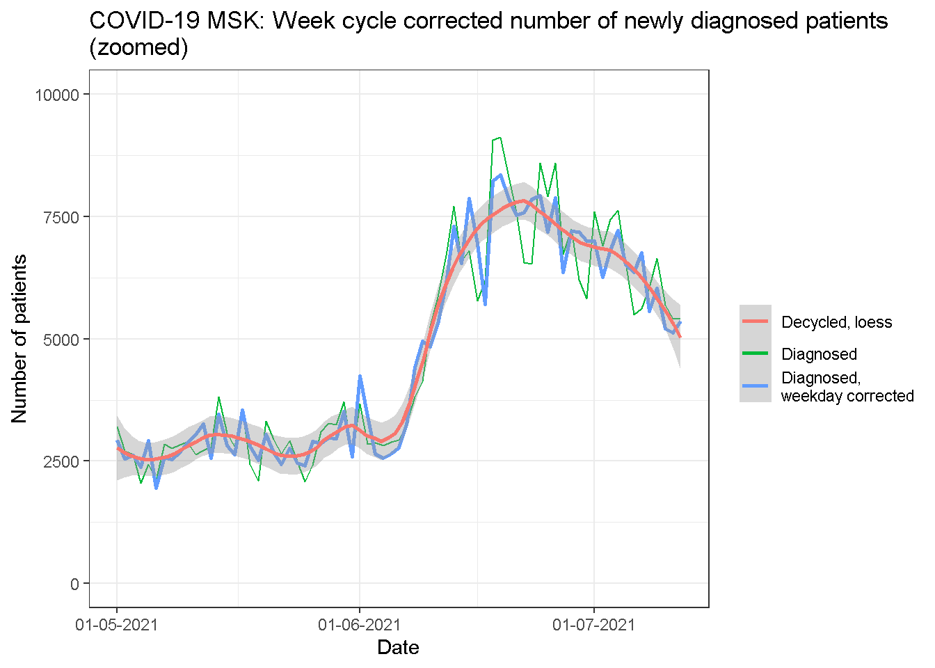
Cyclicity estimates
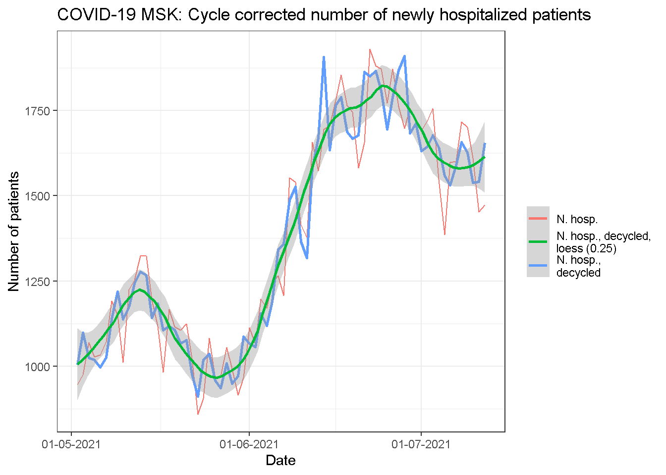
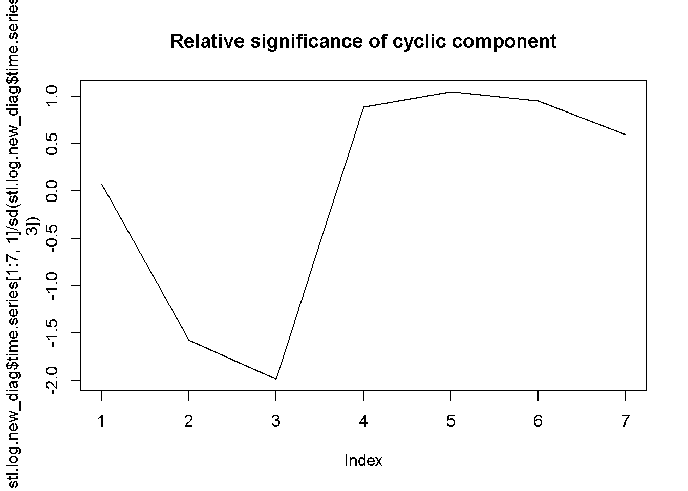
## Weekly diag. cyclicity coeffs:; 1.01; 0.86; 0.83; 1.09; 1.10; 1.09; 1.06
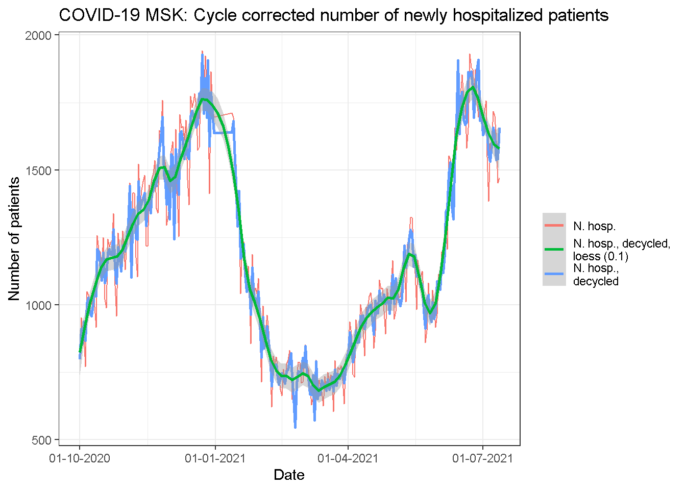
## Weekly hosp. cyclicity coeffs:; 0.89; 1.04; 1.01; 1.04; 1.05; 1.05; 0.94
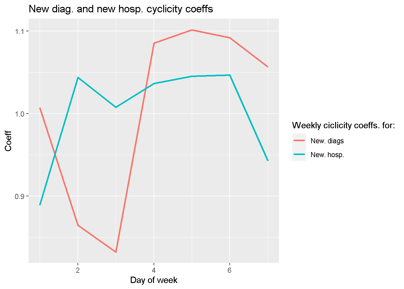
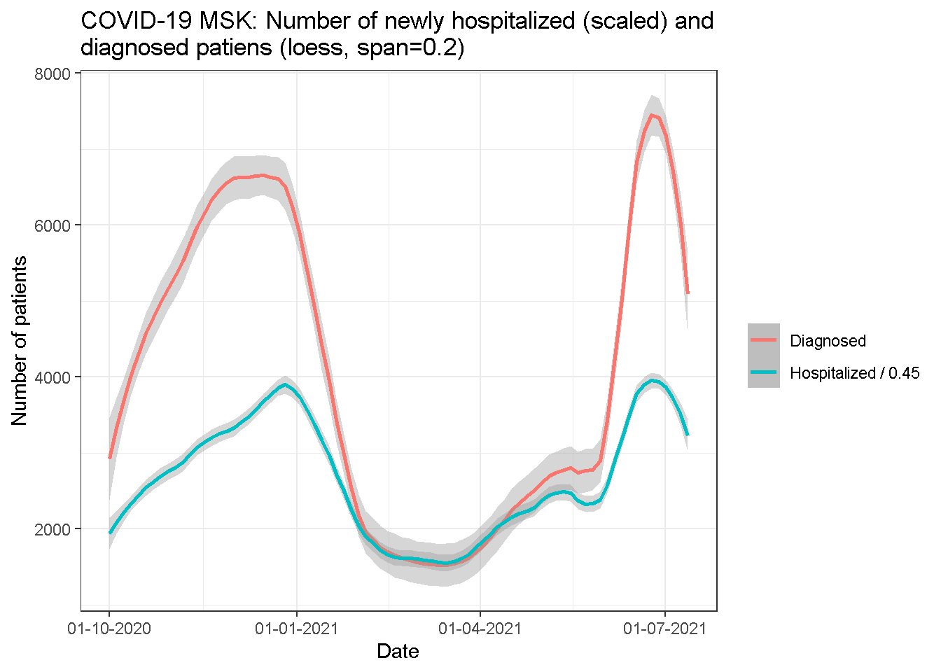
From cyclicity coeffs we may guess that hospitalizations are really 5 days lagged relative to newly diagnosted.
Trends
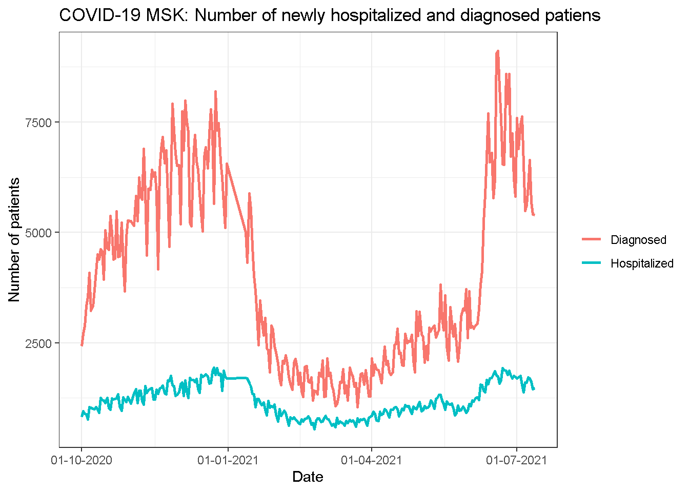
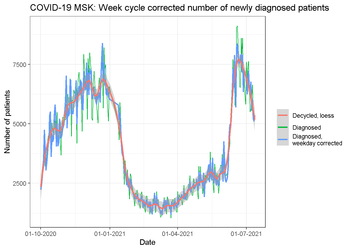
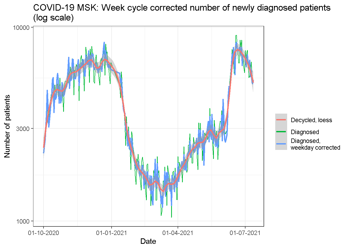
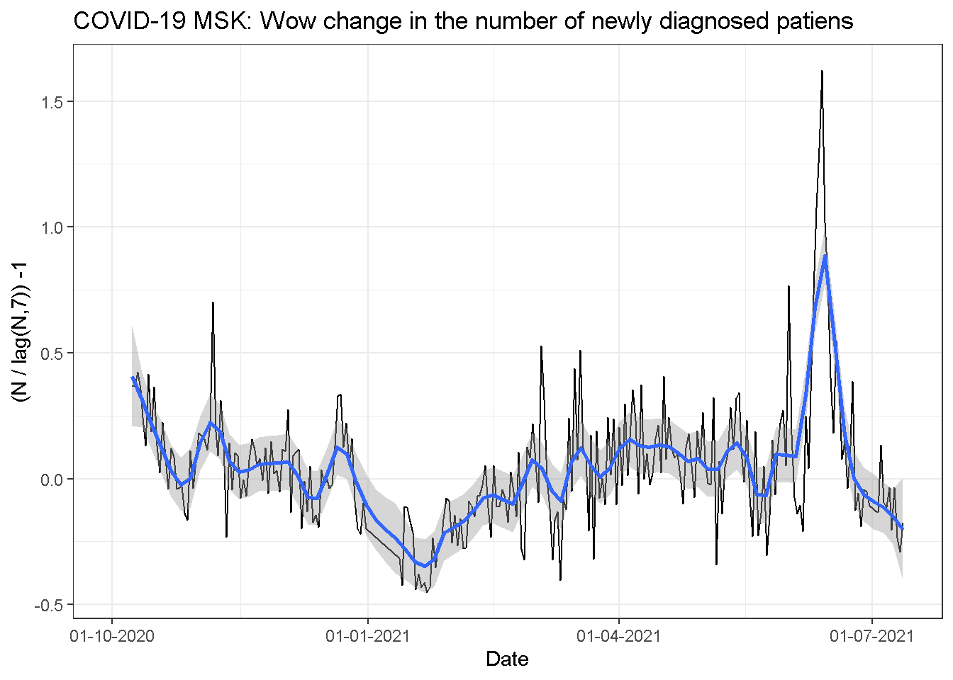
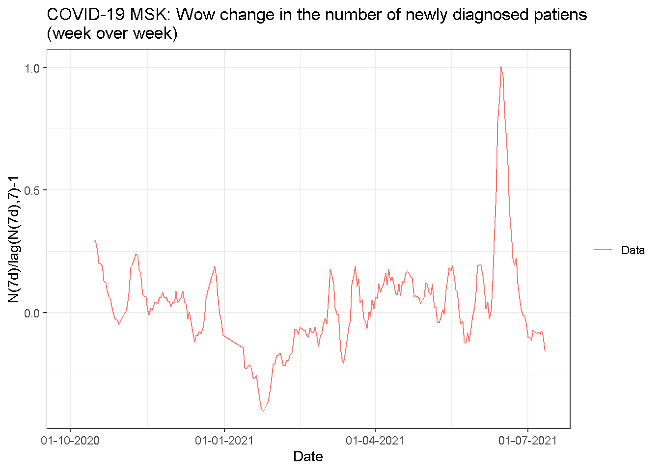
## [1] 266
Latest data table
##          date new_diag new_diag_corr new_diag_week_av new_hosp new_hosp_corr
## 1: 2021-07-06     5498      6360.874         6776.857     1598      1531.055
## 2: 2021-07-07     5621      6754.520         6748.000     1601      1588.553
## 3: 2021-07-08     6040      5563.947         6525.571     1717      1656.384
## 4: 2021-07-09     6643      6029.397         6489.857     1700      1626.196
## 5: 2021-07-10     5694      5214.228         6239.571     1610      1538.209
## 6: 2021-07-11     5410      5119.643         5923.286     1453      1541.010
## 7: 2021-07-12     5403      5363.787         5758.429     1472      1655.919
Newly hospitalized vs. newly disagnosted relationship
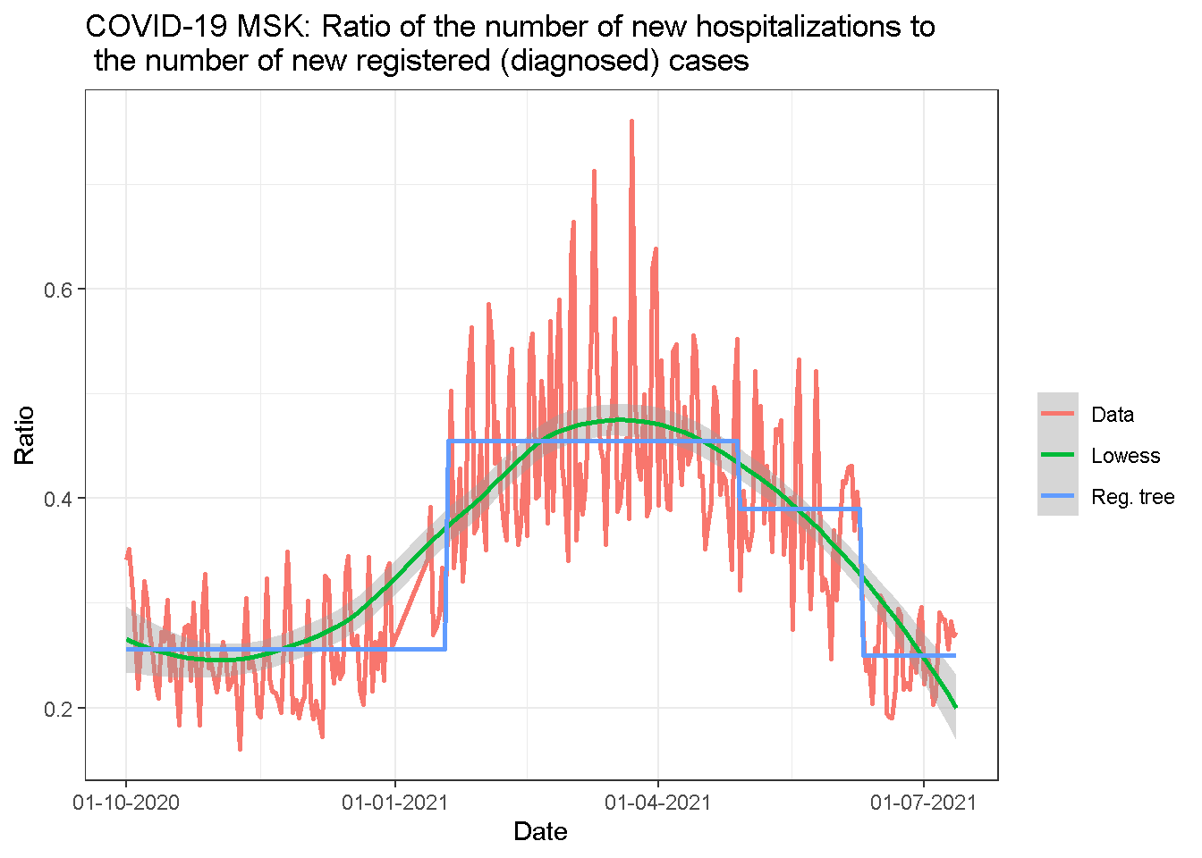
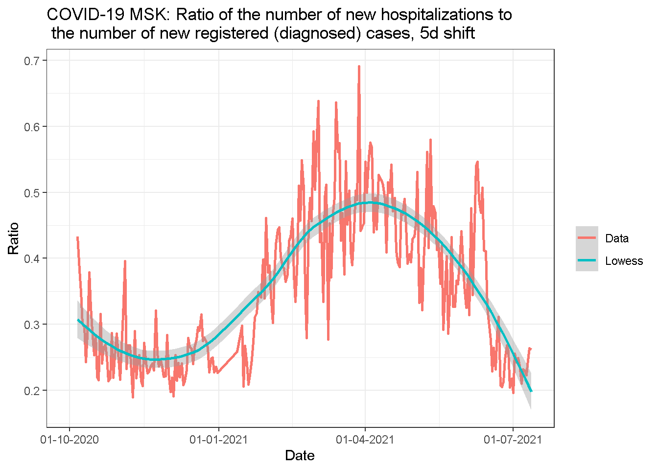
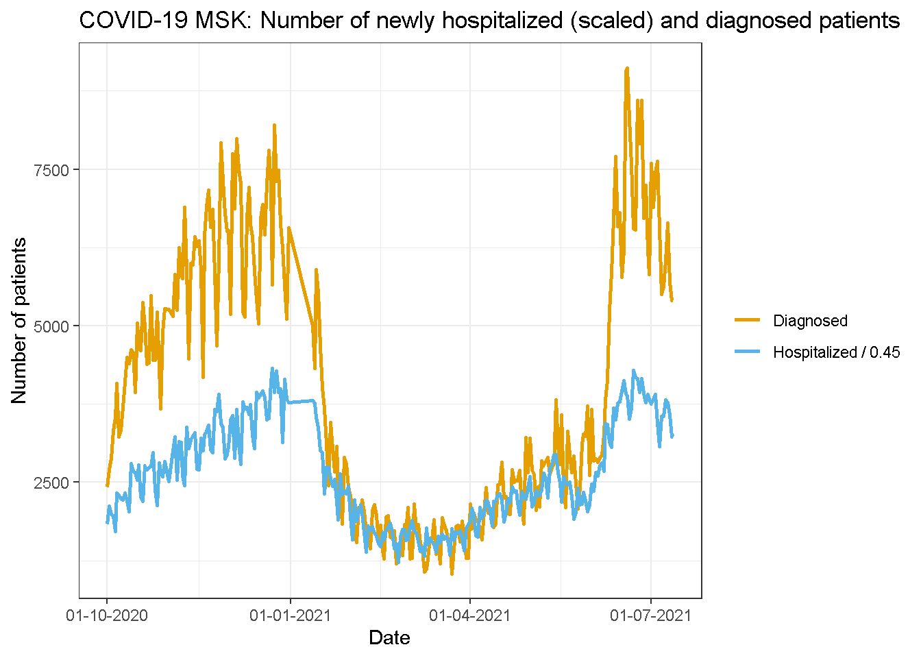
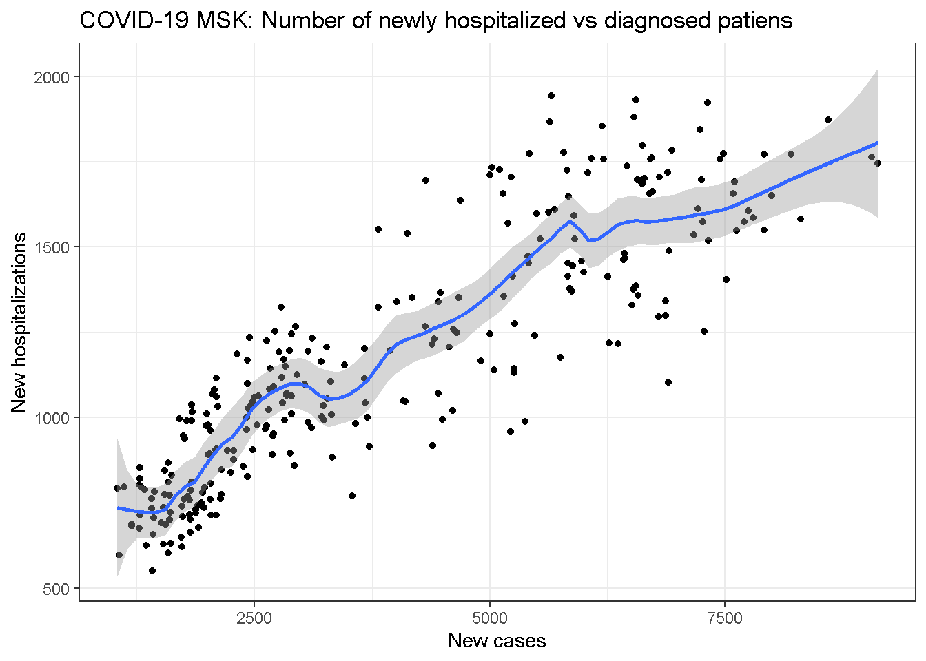
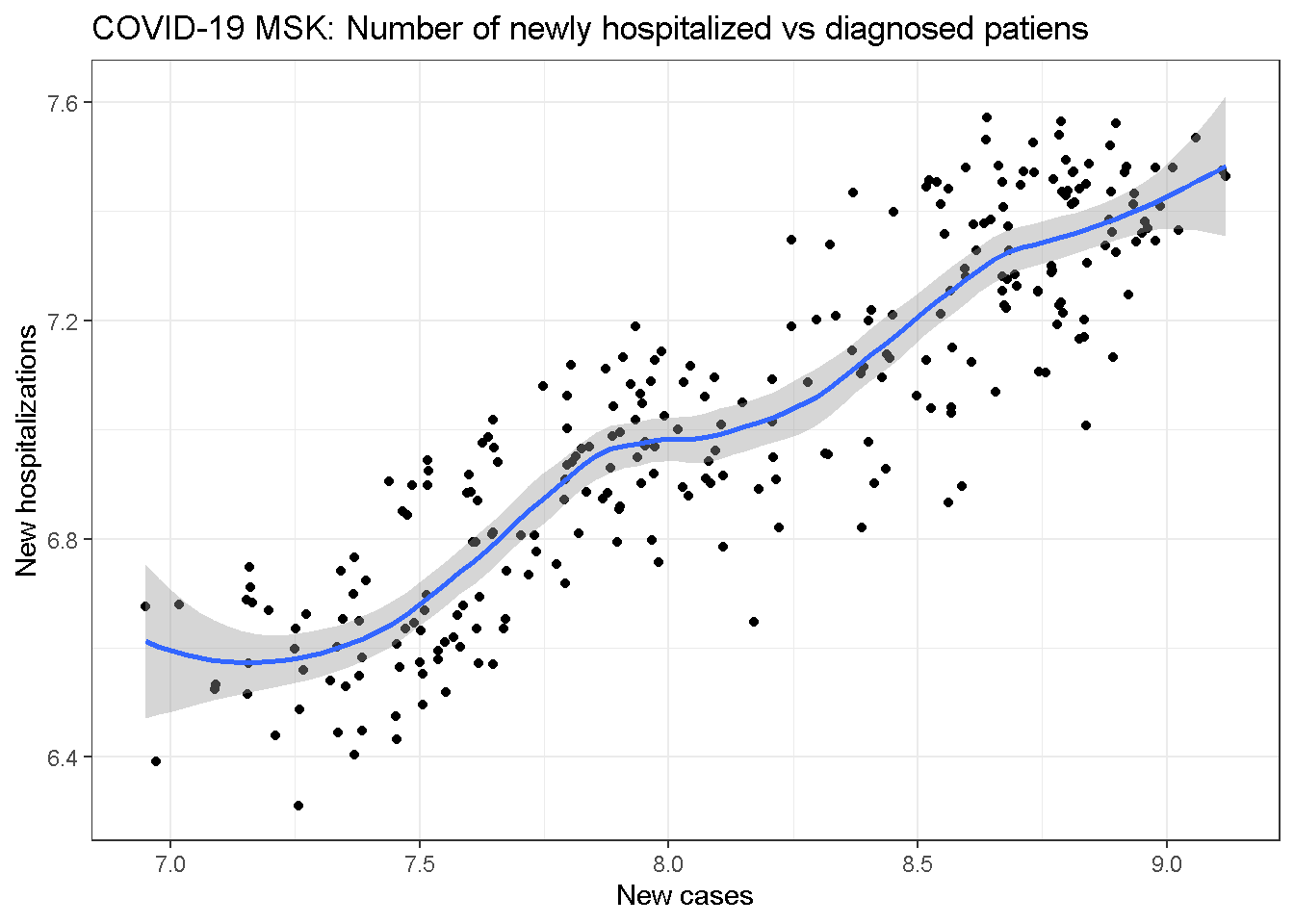
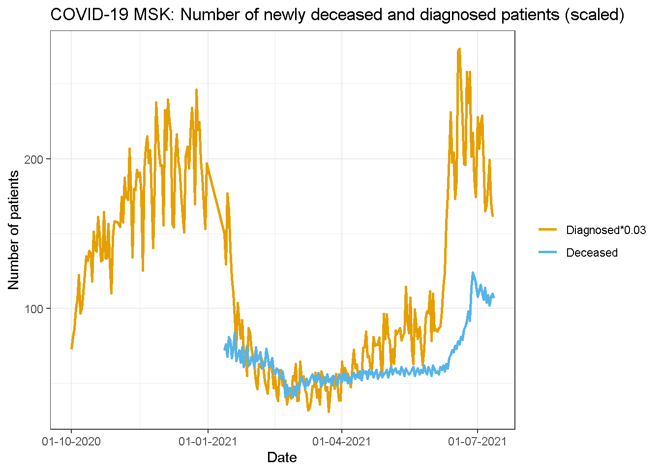
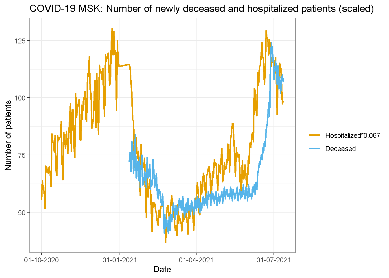
The ratio of the number of hospitalizations to the number of new cases changes with time. The more sick people skip the smaller the ratio.
##
## Call:
## lm(formula = log(new_hosp) ~ log(new_diag), data = dt.data)
##
## Residuals:
##      Min       1Q   Median       3Q      Max
## -0.39739 -0.09287  0.00199  0.10879  0.29966
##
## Coefficients:
##               Estimate Std. Error t value Pr(>|t|)
## (Intercept)    3.08354    0.12235    25.2   <2e-16 ***
## log(new_diag)  0.48483    0.01501    32.3   <2e-16 ***
## ---
## Signif. codes:  0 '***' 0.001 '**' 0.01 '*' 0.05 '.' 0.1 ' ' 1
##
## Residual standard error: 0.1415 on 270 degrees of freedom
## Multiple R-squared:  0.7944,	Adjusted R-squared:  0.7937
## F-statistic:  1043 on 1 and 270 DF,  p-value: < 2.2e-16
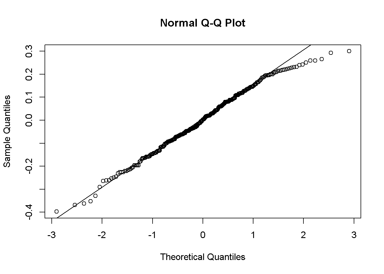
The same is true for deceased time series.
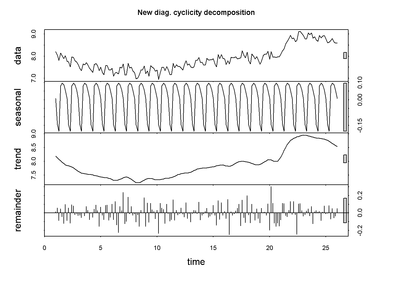
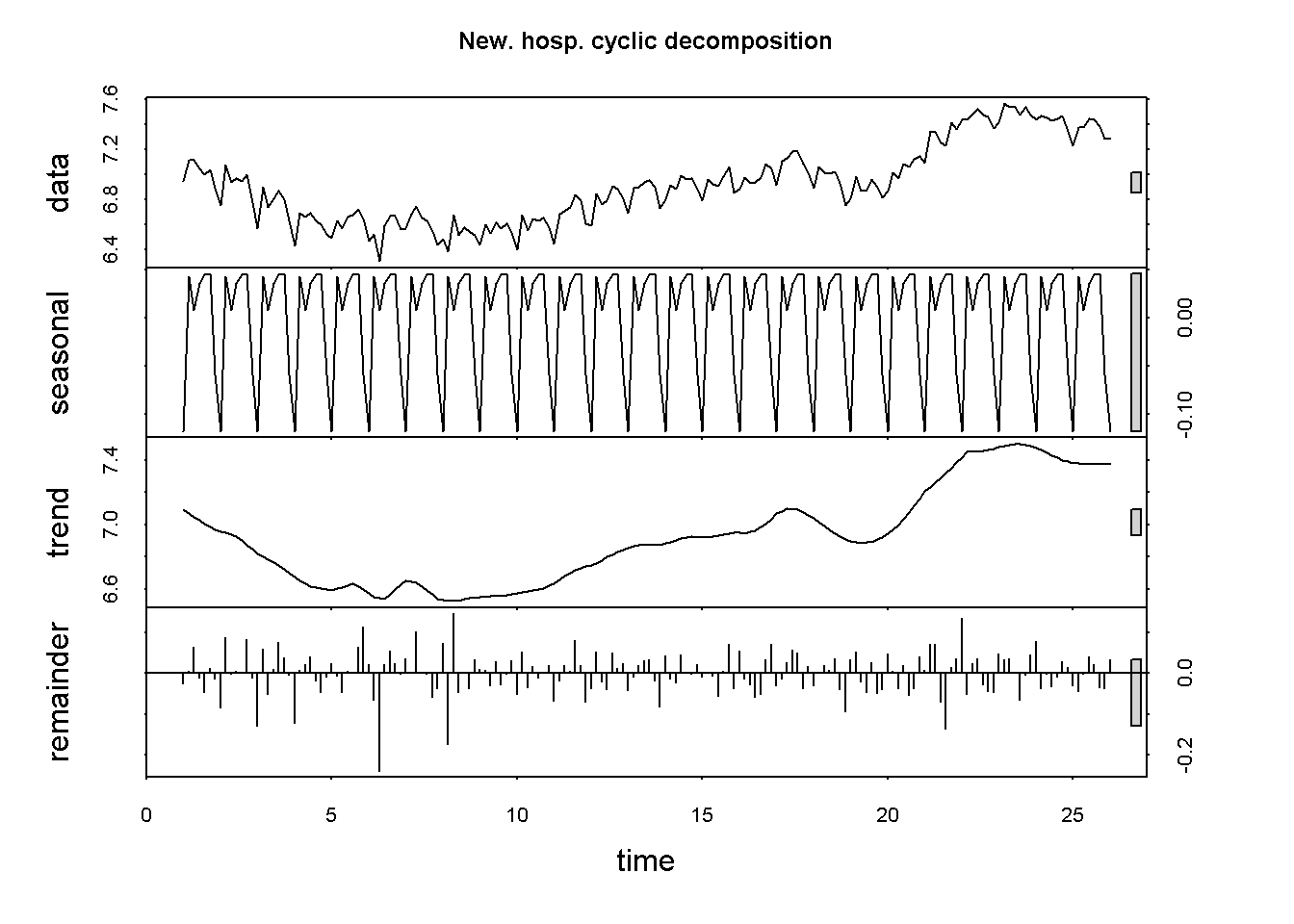
Cyclicity decomposition diagnostic plots
## [1] 0.09251658
## Time Series:
## Start = c(25, 3)
## End = c(26, 1)
## Frequency = 7
## [1] 6754.520 5563.947 6029.397 5214.228 5119.643 5363.787
## [1] 6754.520 5563.947 6029.397 5214.228 5119.643 5363.787
## Time Series:
## Start = c(25, 3)
## End = c(26, 1)
## Frequency = 7
## [1] 6200.499 5958.283 5725.529 5509.639 5301.891 5100.808
ACF Plots
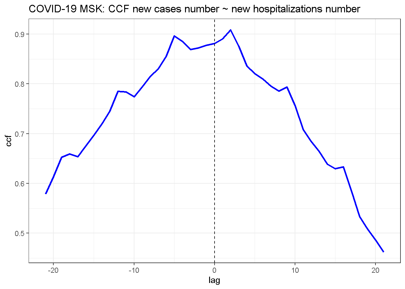
No clear indication for a time lag between the two series. However cross correlation function is more biases towards negative lags as it should be: diagnostic sightly precedes hospitalizations.
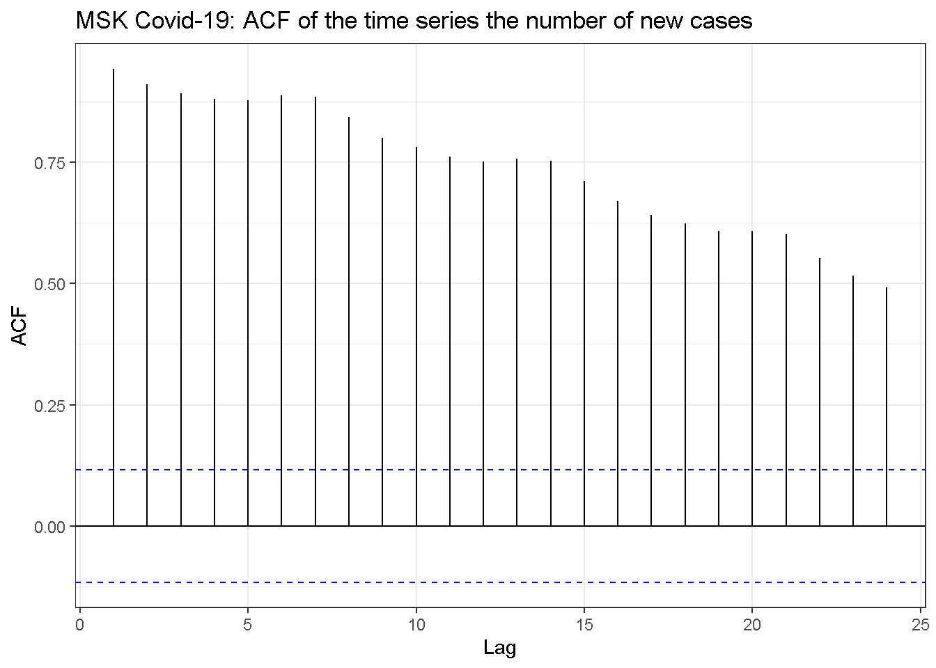
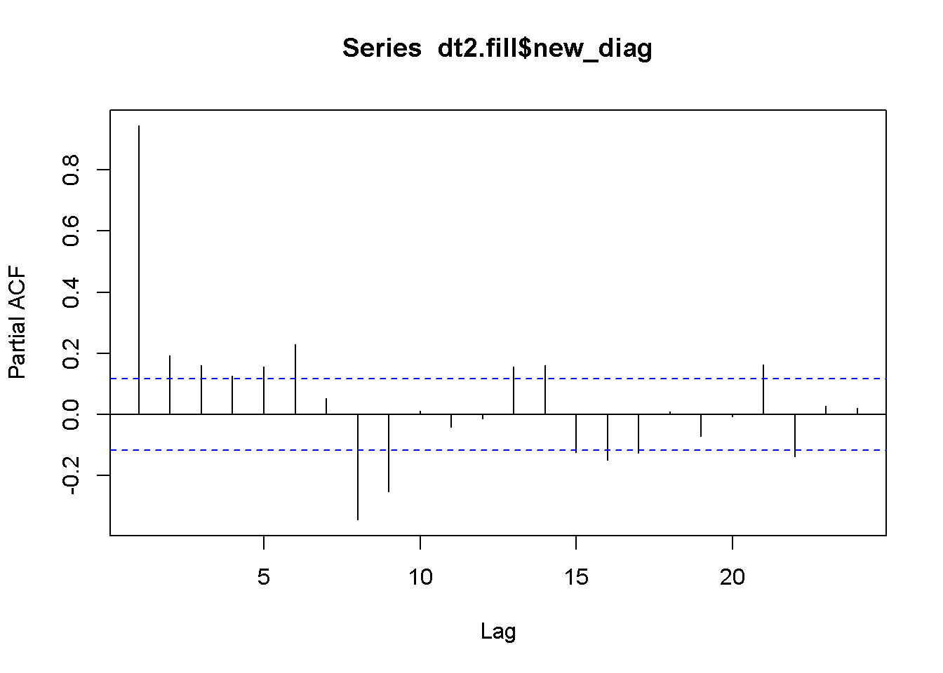
No indication for periodicity in the auto correlation function (same is in logs).
Author Vladislav Borkus
LastMod 2021-07-12
License (C) Vladislav Borkus